セグメンテーションを、市販のソフトのボタンではなく自分で書いたコードで行い、さらに深層学習のモデルに任せるまでの道筋をたどる章である。理論はセグメンテーションの理論の章にあり、ここではそれが実際のコードでどう動くかを見る。
要点は、規則を書くか(しきい値)、例から学ばせるか(CNN・U-Net)の違いと、どちらでも結果を人が確かめることである。
- プログラミングと Python — 道具を借りて組み立てる
- 作業環境 — 手元の計算機か、クラウドか、院内のサーバか
- DICOM を読む — 画素値を HU に戻し、スライスを積み上げる
- しきい値のコード — 肺を取り出す4つの段階
- コマンド型とモデル型 — 規則を書くか、例から学ばせるか
- CNN と U-Net — 画像を見るための網
- 学習済みモデルで臓器を分ける — 前処理・推論・後処理、そして体積
プログラミングと Python — 道具を借りて組み立てる
プログラミングとは、データに対して何をするかを手順(アルゴリズム)として書き、計算機に実行させることである。アルゴリズムは料理のレシピや取扱説明書と同じ「決まった順に行えば決まった結果になる手続き」で、それを計算機が読める形式の言語で書いたものがプログラムになる。
医用画像の処理で Python が選ばれる理由は4つにまとまる。①文法が単純で、プログラマでない医療者でも読める。②ライブラリが膨大で、画像処理・統計・機械学習の部品がすでにある。③データ解析・可視化・機械学習・作業の自動化を1つの言語でこなせる。④利用者が多いので、困ったときの情報と求人が多い。
ライブラリは「特定の目的の関数を集めた道具箱」である。数値の配列を扱う numpy、表を扱う pandas、グラフを描く matplotlib・seaborn、DICOM を読む pydicom、画像処理の scikit-image などを、pip install で入れてから import で読み込む。import pandas as pd のように短い別名を付けるのが慣習で、以後のコードが短く読みやすくなる。
なぜ自分でコードを書く必要があるのか。市販のセグメンテーションソフトはボタンで同じことができるが、手順が画面の操作として残るだけで、他人が同じ結果を再現しにくい。コードなら閾値・順序・パラメータが全部文字として残り、100人分の画像に同じ処理を一度にかけられる。研究で「同じ条件で処理した」と言えるのはこのためである。
ライブラリを使うときの心得は、中で何が起きているかを1文で言えるものだけ使うことである。関数名を並べるだけでは結果の誤りに気づけない。
English version
Core
Programming means writing the steps (an algorithm) to be done on data, and letting a computer run them. An algorithm is like a recipe: the same steps in the same order give the same result.
Python is chosen for medical image work for four reasons: ① simple grammar that non-programmers can read, ② a huge number of libraries for image processing, statistics and machine learning, ③ one language covers data analysis, plotting, machine learning and automation, ④ many users, so help is easy to find.
A library is a toolbox of functions for one purpose: numpy (number arrays), pandas (tables), matplotlib / seaborn (plots), pydicom (DICOM files), scikit-image (image processing). You install it with pip install and load it with import. A short alias such as import pandas as pd keeps later code short.
Going further
Why write code at all? Commercial software can do the same with buttons, but the steps stay only as clicks, so others cannot easily repeat the result. In code, every threshold, order and parameter is written down, and the same process can run on 100 patients at once. This is what makes research reproducible.
A good rule: only use a library function if you can say in one sentence what it does inside. Otherwise you will not notice when the result is wrong.
作業環境 — 手元の計算機か、クラウドか、院内のサーバか
Python を動かす場所は大きく3つある。
| Anaconda+Jupyter | Google Colab | 大学・病院の計算サーバ(JupyterHub) | |
|---|---|---|---|
| どこで動く | 自分の計算機に入れる | ブラウザから Google のサーバ | 施設内の高性能サーバ(GPU つき) |
| データ | 手元のファイルをそのまま使える | アップロードが必要。どの端末からも開ける | 施設内に置いたまま使える |
| 速さ | 自分の計算機の性能次第 | 回線と割り当て次第 | 大きな3D データ・深層学習に向く |
Anaconda は Python と科学計算用ライブラリをまとめた配布版で、ライブラリ同士の版の食い違いを conda が管理する。インストール後は、コマンドプロンプトで python -V や conda -V と打って版が表示されれば準備完了である。Jupyter はブラウザ上の統合開発環境(IDE)で、コードをセルに分けて1つずつ実行し、その場に画像やグラフを出せる。Colab も同じノートブック形式で、主なライブラリが最初から入っている(!pip freeze で一覧を確かめられる)。OS による画面の違いに悩まず全員が同じ画面で学べる点も Colab の利点である。
なぜノートブック形式が画像処理に向くのか。閾値を1つ変えるたびに結果の断面を目で確かめる、という試行錯誤が処理の本体だからである。セルごとに実行して途中の画像を残せるので、どの段階で失敗したかが一目で分かる。
ファイルの読み込みは、ノートブックと同じフォルダにあればファイル名だけで、別の場所ならフルパスで指定する。読み込めないときの原因の大半はこの場所の指定である。
患者の画像をどこで処理するかは、技術ではなく個人情報の問題である。DICOM ファイルには画像だけでなく、患者の氏名・ID・生年月日・撮影日などがヘッダとして入っている。これを外部のクラウドに上げれば、個人データを施設の外に出すことになる(EU では GDPR、日本では個人情報保護法の対象)。教育用の公開データや匿名化したデータでない限り、施設内のサーバで処理するのが原則である。
English version
Core
There are three main places to run Python: (1) Anaconda + Jupyter installed on your own computer — files are used directly, speed depends on your computer; (2) Google Colab in the browser on Google’s servers — data must be uploaded, and it opens from any device; (3) a high-performance server of the university or hospital (JupyterHub, with GPU) — good for large 3D data and deep learning, and data stays inside.
Anaconda is a Python distribution with scientific libraries; conda manages library versions. After install, typing python -V or conda -V should show a version. Jupyter is a browser-based IDE: code is split into cells that run one by one, and images and plots appear right there. Colab uses the same notebook style and already has the main libraries (!pip freeze lists them). Everyone sees the same screen, whatever their operating system.
Going further
Why notebooks suit image work: the real work is trial and error — change a threshold, look at the slice again. Running cell by cell keeps every middle image, so you can see where it went wrong.
To load a file: if it is in the same folder as the notebook, the file name is enough; otherwise give the full path. Most loading errors come from this.
In the clinic
Where you process patient images is a privacy question, not a technical one. A DICOM file holds not only the image but also a header with the patient’s name, ID, birth date and scan date. Uploading it to an outside cloud moves personal data out of the hospital (GDPR in the EU; the Act on the Protection of Personal Information in Japan). Unless the data are public teaching data or anonymised, process them on the hospital’s own server.
DICOM を読む — 画素値を HU に戻し、スライスを積み上げる
CT の1枚1枚は DICOM ファイルで、ヘッダ(撮影条件・患者情報)と画素の配列が1つになっている。pydicom でファイルを読むと、画素は pixel_array(512×512 の数の表)として取り出せる。
ただし保存されている数はそのままでは CT 値ではない。容量を節約するため縮めた整数で記録されているので、ヘッダの2つの値で戻す。HU = 保存値 × RescaleSlope + RescaleIntercept。これをしないと閾値を HU で決められない(空気 −1000・水 0 という物差しが使えない)。
3D にするには、フォルダの全スライスを読んで正しい順に並べ、1つの3次元配列に積む。フォルダからファイルを読み出す順番は位置の順とは限らないので、ヘッダのスライス番号(InstanceNumber)やスライスの位置で並べ替えてから、512×512×枚数の配列に入れる。こうしてできた配列は、どの軸で切るかを変えるだけで横断面・冠状断面・矢状断面のどれでも表示できる。表示には matplotlib を使い、灰色の濃淡(グレースケール)で描いて横に HU の目盛りを付ける。
なぜ並べ替えが要るのか。順番を間違えて積んでも計算機はエラーを出さず、ずれた3D モデルが黙ってできあがる。断面を何枚か並べて表示し、頭側から尾側へ順に変わっていくことを目で確かめるのが最初の検証になる。
画素の大きさ(PixelSpacing)とスライスの厚さ・間隔もヘッダにある。面内が 0.7 mm でスライスが 3 mm なら、ボクセルは縦長の直方体で、配列の1目盛りは方向によって長さが違う。体積や距離を測るときは必ずこの値を掛ける(等方性ボクセルの話と同じ問題)。専用の医用画像ライブラリは、読み込み時に向き(左右・前後・上下)をそろえ、この間隔の情報を画像に付けたまま運んでくれる。
English version
Core
Each CT slice is a DICOM file: a header (scan settings, patient data) plus an array of pixels. With pydicom the pixels come out as pixel_array, a 512×512 table of numbers.
These stored numbers are not yet CT values. They are saved as compact integers, so you convert them with two header values: HU = stored value × RescaleSlope + RescaleIntercept. Without this you cannot set a threshold in HU (air −1000, water 0).
For 3D, read all slices in the folder, sort them into the right order, and stack them into one 3D array (512×512×number of slices). Files are not read in position order, so sort by the slice number in the header (InstanceNumber) or by slice position. The array can then be cut along any axis to show axial, coronal or sagittal planes. matplotlib draws them in grey scale with an HU colour bar.
Going further
Why sorting matters: if slices are stacked in the wrong order, the computer gives no error — it quietly builds a wrong 3D model. Showing several slices in a row and checking that they change smoothly from head to feet is the first check.
Pixel size (PixelSpacing) and slice thickness are also in the header. If pixels are 0.7 mm and slices 3 mm, each voxel is a tall box, and one array step means a different length in each direction. Always multiply by these values when you measure volume or distance (the same issue as isotropic voxels). Medical imaging libraries can fix the orientation (left–right, front–back, up–down) on loading and carry the spacing with the image.
しきい値のコード — 肺を取り出す4つの段階Pulmo
コードで行うセグメンテーションのいちばん単純な例が、胸部 CT から肺 Pulmo(肺)を取り出す処理である。流れは4段階になる。
①しきい値を決めて二値化する。HU のヒストグラム(値ごとの画素数)を描くと、−1000 付近(空気と肺)と 0 付近(軟部組織)に2つの山ができる。大津の方法(Otsu)は、2つの群それぞれのばらつきが最小になる位置、つまり山と山の谷に自動で線を引く。その線より低い画素を 1、高い画素を 0 にすると白黒の画像(二値画像)ができる。
②縁に接する領域を消す(clear_border)。体の外の空気も肺と同じく低い値なので一緒に拾われる。体外の空気は画像の縁につながっているので、縁に触れる塊を除けば肺だけが残る。
③小さな島を消す(remove_small_objects)。一定の画素数より小さい塊は、腸管のガスや雑音とみなして捨てる。
④穴を埋め、輪郭を滑らかにする(binary_closing、円盤形の構造要素)。肺の中の血管は軟部組織の値なので、二値画像では肺に開いた黒い穴になる。膨張してから収縮するクロージングで、小さな穴と輪郭のぎざぎざを埋める。
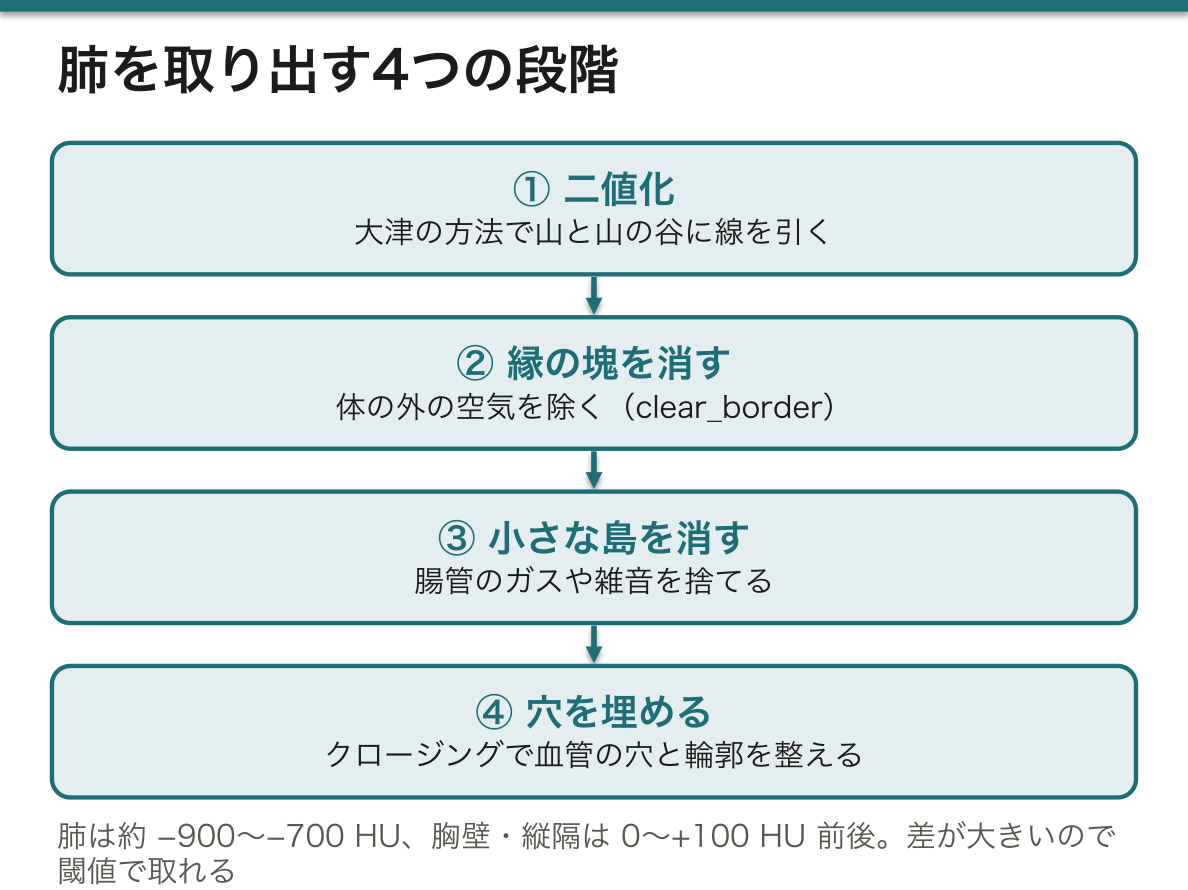
なぜ肺はしきい値だけで取れるのか。肺は大部分が空気で、およそ −900〜−700 HU にあり、周りの胸壁・縦隔(0〜+100 HU 前後)との差が数百 HU もある。肝と脾のように値が重なる臓器ではこうはいかない(閾値法の限界)。
④の円盤の大きさは結果を変える。大きくすると血管の穴はきれいに埋まるが、肺の縁の細かいくぼみまで埋まって体積が増える。パラメータは見た目ではなく、測りたいものに合わせて決める。また気管と主気管支も空気なので同じ値で拾われる。肺だけが欲しいなら、これを別に切り離す処理が要る。
肺の自動セグメンテーションは、肺気腫の定量(−950 HU 未満の領域が肺全体の何%か)や、肺結節の検出の前処理、放射線治療で守るべき臓器としての肺の輪郭作りに使われている。
English version
Core
The simplest example of segmentation by code is taking the lung (Pulmo) out of a chest CT. There are four steps.
① Threshold and binarise. The HU histogram has two peaks: near −1000 (air and lung) and near 0 (soft tissue). Otsu’s method draws the line automatically in the valley, where the spread inside each group is smallest. Pixels below the line become 1, the rest 0 — a black-and-white (binary) image.
② Remove regions touching the border (clear_border). Air outside the body is also low and is picked up too, but it touches the edge of the image, so removing border-touching blobs leaves the lungs.
③ Remove small islands (remove_small_objects): blobs smaller than a set size are treated as bowel gas or noise.
④ Fill holes and smooth the outline (binary_closing with a disc). Vessels inside the lung have soft-tissue values and appear as holes. Closing (dilate, then erode) fills small holes and rough edges.
Going further
Why does a threshold alone work for the lung? The lung is mostly air, about −900 to −700 HU, and the chest wall and mediastinum (around 0 to +100 HU) differ by several hundred HU. For organs with overlapping values, like liver and spleen, this fails (limits of thresholding).
The disc size in ④ changes the result: a larger disc fills vessel holes well but also fills small dents at the lung edge, so the volume grows. Choose parameters for what you want to measure, not for the look. The trachea and main bronchi are also air and are picked up too; to get only the lungs they must be cut off separately.
In the clinic
Automatic lung segmentation is used to measure emphysema (the % of lung below −950 HU), as a first step in finding lung nodules, and to outline the lungs as an organ to protect in radiotherapy.
コマンド型とモデル型 — 規則を書くか、例から学ばせるか
前の項目の肺の処理はコマンド型(規則に基づく)セグメンテーションである。人が「−500 HU より低く、縁に触れず、200 画素より大きい」という規則を書き、計算機はそれに従うだけである。速く、なぜそう分けたかを説明できるが、規則で書けない対象(値が重なる軟部組織、形の個人差)には使えない。
モデル型では規則を書かない。正解の輪郭を付けた画像を大量に見せ、入力から正解を出す関数そのものを学習させる。その中身がニューラルネットワークである。
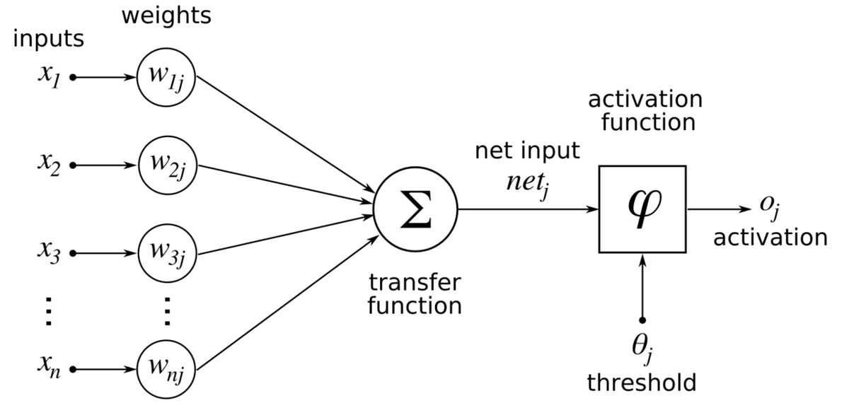
最小単位の人工ニューロンは、入力 x1…xn にそれぞれ重み w を掛けて足し(h = Σ xiwi)、その和を活性化関数 f に通して出力 y = f(h) を出す。これを層にして並べ、入力層 → 隠れ層 → 出力層とつないだものがネットワークになる。
学習とは重みを決めることである。①ネットワークに画像を入れて出力を出す ②正解との差(誤差)を計算する ③誤差を出力側から入力側へさかのぼって、各重みをどちらにどれだけ動かせば誤差が減るかを求める(誤差逆伝播法 back-propagation)④重みを少し直す。これを何万回も繰り返す。
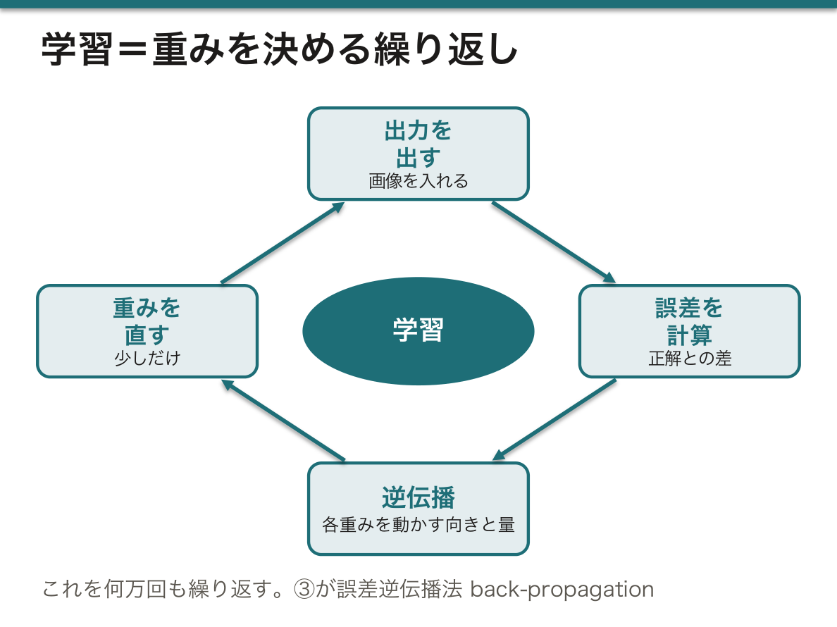
なぜ活性化関数が要るのか。掛けて足すだけの操作は何層重ねても1回の掛け算と足し算にまとめられてしまい、直線的な区別しかできない。間に「0 より小さければ 0」(ReLU)のような折れ曲がりを挟むことで、層を重ねるほど複雑な境界を表せるようになる。
モデル型の弱点は、規則が重みの中に分散していて人が読めないこと、そして学習データに無い種類の画像(別の装置・まれな病変・金属)で黙って誤ることである。だから臨床ではモデルの出力を人が確かめる半自動が基本になる(セグメンテーションの理論の章の AI の項目)。
English version
Core
The lung pipeline above is rule-based (command-based) segmentation: a person writes the rules (“below −500 HU, not touching the border, larger than 200 pixels”) and the computer follows them. It is fast and explainable, but it fails where rules cannot be written (overlapping soft tissues, shape differences between people).
In the model-based approach, no rules are written. You show many images with correct outlines, and the computer learns the function from input to answer. Inside is a neural network.
The basic unit, an artificial neuron, multiplies each input xi by a weight wi, adds them (h = Σ xiwi), and passes the sum through an activation function: y = f(h). Neurons in layers — input, hidden, output — make a network.
Training means finding the weights: ① feed an image and get an output, ② compute the error against the correct answer, ③ pass the error backwards to find how each weight should change (back-propagation), ④ adjust the weights a little. Repeat many thousands of times.
Going further
Why an activation function? Multiply-and-add, however many layers, collapses into one multiply-and-add, so it can only draw straight boundaries. A bend such as ReLU (“if below 0, give 0”) between layers lets deeper networks draw complex boundaries.
Weak points of models: the rules are spread across the weights, so people cannot read them, and they fail quietly on images unlike the training data (other scanners, rare lesions, metal). That is why clinical use is semi-automatic, with a person checking the output (see the AI item in the chapter on segmentation theory).
CNN と U-Net — 画像を見るための網
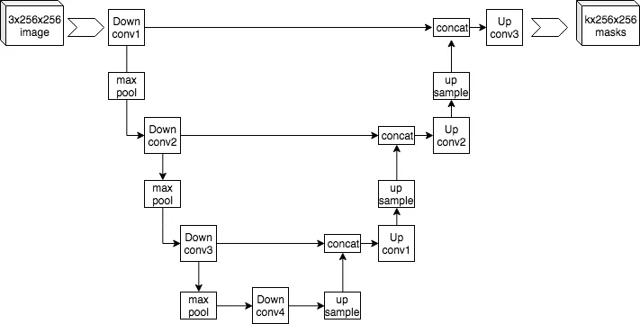
画像をそのまま普通のネットワークに入れると、512×512 の画素1つ1つに別々の重みが要り、しかも隣り合う画素の関係が無視される。畳み込みニューラルネットワーク(CNN)はこれを解決した。
畳み込みでは、3×3 などの小さな重みの窓(カーネル)を画像の上で1画素ずつずらし、窓の下の画素と重みを掛けて足した値を新しい画像に書く。たとえば左列が +1・右列が −1 のカーネルは、左右で明るさが変わる所、つまり縦の輪郭で大きな値を出す。縁に 0 を足して(パディング)おけば出力は元と同じ大きさになる。こうしてできた画像が特徴マップである。次にプーリング(2×2 の中の最大値だけ残すなど)で縦横を半分にする。
これを重ねると、浅い層は輪郭、中間の層は輪郭の組み合わせ(部品)、深い層は物の形に反応するようになる。カーネルの値は人が決めるのではなく、学習で決まる。
セグメンテーションでは「何が写っているか」ではなく画素ごとのラベルが要る。U-Net は、畳み込みとプーリングで縮めていくエンコーダ(何があるかをつかむ)と、拡大して元の大きさに戻すデコーダ(どこにあるかを描く)を U 字につなぎ、同じ解像度の段どうしをスキップ接続で直結した構造である。
なぜスキップ接続が要るのか。縮める途中で「ここは肝臓らしい」という意味は強くなるが、正確な位置の情報は失われる。拡大するだけでは輪郭がぼやける。縮める前の細かい特徴マップを拡大側へそのまま渡すことで、意味(何か)と位置(どこか)を両立させている。
U-Net が医用画像で標準になったのは、もともと生物医学画像のために作られ、正解付きの画像が少なくても学習できるよう設計されていたからである。正解の輪郭を描けるのは専門家だけなので、医用画像では学習データが常に足りない。CT の 3D データには、立方体のカーネルを使う 3D 版が使われる。
English version
Core
Putting a whole image into a plain network needs a separate weight for every one of 512×512 pixels and ignores which pixels are neighbours. The convolutional neural network (CNN) solves this.
In convolution, a small window of weights (a kernel, e.g. 3×3) slides across the image; at each place the pixels under it are multiplied by the weights and added, and the result goes into a new image. A kernel with +1 on the left column and −1 on the right gives large values where brightness changes left to right — a vertical edge. Adding zeros around the border (padding) keeps the output the same size. The output is a feature map. Then pooling (e.g. keep the maximum of each 2×2) halves the size.
Stacked, early layers respond to edges, middle layers to combinations of edges (parts), deep layers to whole shapes. The kernel values are learned, not set by people.
Segmentation needs a label for every pixel, not just “what is in the image”. U-Net joins an encoder that shrinks the image (finding what) and a decoder that enlarges it back (drawing where) in a U shape, with skip connections linking levels of the same resolution.
Going further
Why skip connections? While shrinking, the network learns meaning (“this looks like liver”) but loses exact position; enlarging alone gives blurred outlines. Passing the fine feature maps straight across to the decoder keeps both meaning and position.
U-Net became the standard for medical images because it was built for biomedical images and designed to learn from few labelled images. Only experts can draw correct outlines, so medical training data are always short. For 3D CT, a 3D version with cube-shaped kernels is used.
学習済みモデルで臓器を分ける — 前処理・推論・後処理、そして体積
自分でネットワークを学習させなくても、公開されている学習済みモデルを使えば全身 CT から多数の臓器を一度に分けられる。医用画像の深層学習用には、PyTorch を土台にした MONAI というライブラリ群があり、学習済みモデルの置き場(model zoo)も用意されている。
使う流れは3段階である。①前処理:DICOM のフォルダを読み込み、チャンネルの次元を先頭にそろえ、向きを決まった座標系(たとえば LPS)に直す。モデルは学習したときと同じ形・向き・値の範囲のデータしか正しく扱えないので、ここで条件を合わせる。②推論:保存されている重みをモデルに読み込み、学習ではなく評価のモードにして画像を通す。全身 CT は一度に入らないので、96×96×96 ボクセルほどの立方体に区切って順に通し、つなぎ合わせる。③後処理:出力を臓器ごとの番号のついたマスク(ラベル画像)に戻す。
マスクができれば数字が出る。臓器の体積 = その番号のボクセル数 × ボクセル1個の体積(3方向の間隔の積)で、たとえば膀胱の容量が cm³ で求まる。
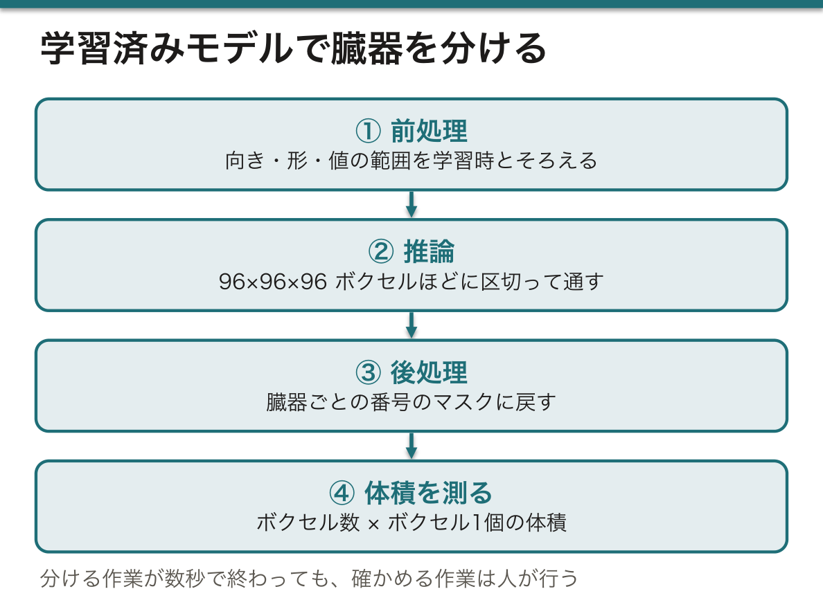
なぜ前処理を学習時とそろえる必要があるのか。モデルは「この向き・この値の範囲で、肝臓はこう見える」という経験しか持っていない。左右が反転した画像や、HU に戻していない値を入れても、モデルはエラーを出さずに見当違いのマスクを返す。学習済みモデルの多くが設定ファイルに前処理の手順を一緒に収めているのはこのためである。
結果の確認には、元の CT とマスクを同じ断面で並べて表示する。分ける作業が数秒で終わっても、確かめる作業は人が行う点は変わらない。
臓器のマスクの使い道は広い。放射線治療計画では、腫瘍に線量を集めつつ避けるべき臓器(リスク臓器)の輪郭を描く作業に使われ、手作業で数時間かかっていた輪郭作りが短くなる。ほかに、PET・SPECT の定量(臓器の範囲を正しく決めて集積を測る)、臓器体積の経過観察、そして3Dプリント用モデルの下書きにもなる。
English version
Core
You do not have to train a network yourself: a public pretrained model can split a whole-body CT into many organs at once. MONAI, a set of libraries built on PyTorch for medical deep learning, offers a model zoo.
Three stages: ① Pre-processing — load the DICOM folder, put the channel dimension first, and turn the image into a fixed orientation (e.g. LPS). A model works only on data with the same shape, orientation and value range it was trained on. ② Inference — load the saved weights, switch the model to evaluation (not training) mode, and pass the image through. A whole-body CT does not fit at once, so it is cut into cubes of about 96×96×96 voxels and joined back. ③ Post-processing — turn the output into a mask (label image) with one number per organ.
With a mask you get numbers: organ volume = number of voxels with that label × volume of one voxel (the product of the three spacings), e.g. bladder volume in cm³.
Going further
Why must pre-processing match training? The model only knows “in this orientation and value range, liver looks like this”. A left–right flipped image or values not converted to HU give no error — just a wrong mask. That is why many pretrained models keep the pre-processing steps in their configuration file.
To check, show the CT and the mask side by side in the same plane. Segmentation may take seconds, but checking is still a human job.
In the clinic
Organ masks have many uses. In radiotherapy planning they outline organs at risk, which the dose must avoid while it is focused on the tumour; contouring that took hours by hand becomes faster. They are also used for PET/SPECT quantification (measuring uptake inside correct organ borders), following organ volume over time, and as a first draft of models for 3D printing.
まとめ
| プログラミングと Python — 道具を借りて組み立てる | プログラミングとは、データに対して何をするかを手順(アルゴリズム)として書き、計算機に実行させることである。 |
|---|---|
| 作業環境 — 手元の計算機か、クラウドか、院内のサーバか | Python を動かす場所は大きく3つある。 |
| DICOM を読む — 画素値を HU に戻し、スライスを積み上げる | CT の1枚1枚は DICOM ファイルで、ヘッダ(撮影条件・患者情報)と画素の配列が1つになっている。 |
| しきい値のコード — 肺を取り出す4つの段階 | コードで行うセグメンテーションのいちばん単純な例が、胸部 CT から肺 Pulmo(肺)を取り出す処理である。 |
| コマンド型とモデル型 — 規則を書くか、例から学ばせるか | 前の項目の肺の処理はコマンド型(規則に基づく)セグメンテーションである。 |
| CNN と U-Net — 画像を見るための網 | 画像をそのまま普通のネットワークに入れると、512×512 の画素1つ1つに別々の重みが要り、しかも隣り合う画素の関係が無視される。 |
| 学習済みモデルで臓器を分ける — 前処理・推論・後処理、そして体積 | 自分でネットワークを学習させなくても、公開されている学習済みモデルを使えば全身 CT から多数の臓器を一度に分けられる。 |
このノートは医学生が授業の内容を自分の言葉でまとめたもので、診療の判断に使うものではありません。誤りに気づいたらお知らせください。