物理の測定は「値」だけでは完結しない。どれだけ信用できるか(不確かさ)と単位がそろって、はじめて他人が使える情報になる。この章では、測った数をどう要約し、どう評価し、どう書くかを扱う。
考え方の芯は2つしかない。ばらつき(精度)とずれ(正確さ)を分けて考えること、そして平均値そのものの不確かさは測定回数を増やすと小さくなること。この2点は臨床検査の基準範囲や精度管理、論文の統計を読むときにもそのまま使う。
式は多く見えるが、平均・標準偏差・標準誤差・信頼区間の4つが一本の流れでつながっている。順番に読めば暗記は要らない。
- 測定値の書き方 — 値・不確かさ・単位の3点セット
- 誤差の種類 — 正確さと精度は別物
- データの要約 — 度数分布と3つの代表値
- 正規分布と標準偏差 — 母集団と標本の違い
- 平均値の信頼区間 — 標準誤差と Student の t
- 結果の評価 — 絶対誤差・相対誤差・相対差
測定値の書き方 — 値・不確かさ・単位の3点セット
測定の目的は、ある物理量(測定量 measurand)について情報を得ることである。結果は必ず①測った値、②不確かさ Δx、③単位の3つで書く。形は x = (x̄ ± Δx) 単位。
1回だけ読んだ値の不確かさは、まず計器の最小目盛(least count)から見積もる。アナログ目盛なら最小目盛かその半分、デジタル表示なら最後の桁の1単位が目安になる。たとえば 5 kg 刻みの体重計で 87 kg と読んだなら、±3 kg 程度の幅を持たせて書くのが正直である。
なぜ値だけではいけないのか。「赤血球の直径は 7.9 μm だった」と言われても、±0.1 μm なのか ±2 μm なのかで意味がまったく違う。前者なら基準値(約 7.5 μm)とのずれは本物の可能性があり、後者なら区別がつかない。比べられるかどうかを決めるのは不確かさのほうである。
書き方の約束も同じ理由から来ている。Δ は有効数字1〜2桁に丸め、平均値は Δ と同じ桁でそろえる。7.4632 ± 0.187 μm ではなく 7.5 ± 0.2 μm と書く。Δ の2桁目より下の数字は、測定が保証していない数字だからである。
体温計・血圧計・体重計など、臨床の計器にも最小目盛と固有の誤差がある。電子体温計の表示は 0.1 ℃ 刻みだが、測り方による差はそれより大きいことが多い。表示の細かさは正確さを保証しない——この区別は、検査値の小さな変動を「変化」と読むかどうかの判断に直結する。
English version
Core
The aim of a measurement is to gain information about a physical quantity, the measurand. A result is always written with three parts: (1) the measured value, (2) the uncertainty Δx, (3) the unit, in the form x = (x̄ ± Δx) unit.
For a single reading, first estimate the uncertainty from the least count of the instrument. For an analog scale, use the smallest division or half of it; for a digital display, use one unit of the last digit. If a scale with 5 kg divisions reads 87 kg, it is honest to write it with a margin of about ±3 kg.
Going further
Why is a value alone not enough? “The red cell diameter was 7.9 μm” means very different things at ±0.1 μm and at ±2 μm. With the first, the difference from the reference value (about 7.5 μm) may be real; with the second, you cannot tell. The uncertainty decides whether two numbers can be compared.
The writing rules follow from the same reason. Round Δ to one or two significant figures, and round the mean to the same decimal place as Δ. Write 7.5 ± 0.2 μm, not 7.4632 ± 0.187 μm. Digits below the second digit of Δ are not supported by the measurement.
In the clinic
Clinical instruments such as thermometers, blood pressure monitors and scales also have a least count and their own errors. An electronic thermometer shows 0.1 °C steps, but the difference caused by how you measure is often larger. A fine display does not guarantee accuracy — this distinction decides whether a small change in a test value should be read as a real change.
誤差の種類 — 正確さと精度は別物
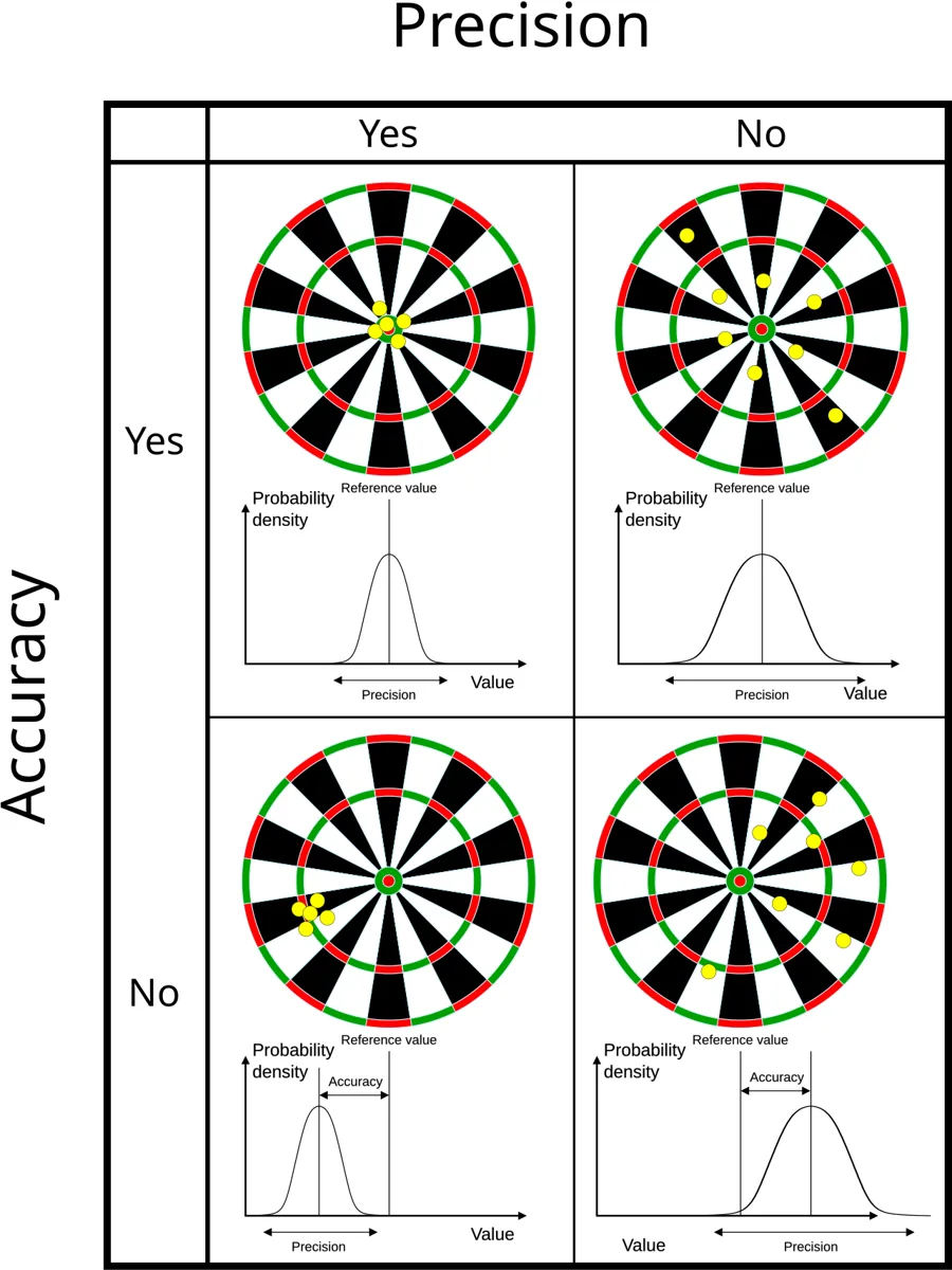
誤差は性質で3つに分ける。
| 種類 | 中身 | 何が落ちるか |
|---|---|---|
| 系統誤差 systematic | いつも同じ向きに同じだけずれる(校正のずれた秤、目盛を斜めから読む癖) | 正確さ accuracy |
| 偶然誤差 random | 毎回ばらばらに散る(読み取りの揺れ、温度や振動のゆらぎ) | 精度 precision |
| 過失誤差 gross | 読み違い・記録ミス。外れ値として現れる | — |
発生源で見ると、計器(instrumental)・観測者(observational)・環境(environmental)・方法そのもの(theoretical)がある。
弓矢のたとえが一番わかりやすい。正確さは矢の集まりの中心が的の中心にどれだけ近いか、精度は矢どうしがどれだけ寄り集まっているか。矢が一か所に固まっていても、的から外れていれば「精度は高いが正確でない」。
なぜ区別が大事か——対処法が逆だからである。偶然誤差は測定を繰り返して平均すれば小さくなる。系統誤差は何回繰り返してもまったく減らない。何も載せないのに −1 kg を示す秤は、100回測っても毎回 1 kg 軽く出る。系統誤差を消すのは校正(基準物で計器を合わせること)だけである。統計的には、精度は標準偏差に、正確さは基準値との差に対応する。
臨床検査の精度管理はこの2軸そのものである。同じ管理試料を毎日測ってばらつき(再現性)を見て、値の分かっている標準物質でかたより(真度)を見る。血圧をカフの細すぎるもので測ると毎回高く出るのは系統誤差の典型で、回数を増やしても直らない。
English version
Core
Errors are divided into three types by their behavior.
| Type | What it is | What it lowers |
|---|---|---|
| Systematic | Always shifts the same way by the same amount (a badly calibrated scale, a habit of reading the scale at an angle) | Accuracy |
| Random | Scatters differently each time (reading fluctuation, changes in temperature or vibration) | Precision |
| Gross | Misreading or recording mistakes; they appear as outliers | — |
By source, errors come from the instrument, the observer, the environment, or the method itself (theoretical).
Going further
The archery picture is the clearest. Accuracy is how close the center of the group of arrows is to the bull’s-eye; precision is how tightly the arrows cluster. Arrows packed in one spot but far from the center are “precise but not accurate”.
Why the distinction matters — the remedies are opposite. Random error shrinks when you repeat the measurement and average. Systematic error does not shrink at all, however many times you repeat. A scale that reads −1 kg with nothing on it gives 1 kg too little every time, even after 100 readings. Only calibration (adjusting the instrument against a known standard) removes systematic error. In statistics, precision corresponds to the standard deviation and accuracy to the difference from the reference value.
In the clinic
Quality control in the clinical laboratory is exactly these two axes. The lab measures the same control sample every day to check spread (reproducibility), and a reference material of known value to check bias (trueness). Measuring blood pressure with a cuff that is too narrow gives a high reading every time — a typical systematic error that repetition does not fix.
データの要約 — 度数分布と3つの代表値
たくさんの測定値は、まず度数分布にまとめる。値を等しい幅の階級に分けて、各階級に入る個数(度数)を数える。度数を全体数で割れば相対度数になる。階級の数の目安には k = 1 + 3.32·log10n(Sturges の式)を使う。
図にする形は3つ:ヒストグラム(階級幅を底辺にした長方形)、度数折れ線(階級の中点を結ぶ)、累積度数(ある値以下の割合)。
代表値は3つある。平均 x̄ = Σx/n、中央値(並べて真ん中。偶数個なら中央2つの平均)、最頻値(いちばん多い値)。
分布が左右対称なら3つは一致する。ずれるのは分布が片側に尾を引くときで、その尾の向きを表すのが歪度(skewness)である。右(大きい値の側)に長く尾を引けば歪度は正で、平均 > 中央値 > 最頻値の順に並ぶ。平均は極端な値に引っ張られるが、中央値は順番しか見ないので動かないからである。
だから分布が対称でないときは中央値を使う。分布の山がとがっているか平たいかは尖度(excess kurtosis)で表し、正規分布で 0 になるよう定義される。
入院日数・医療費・CRP のような検査値は右に長い尾を持つ。「平均入院日数」は少数の長期入院で大きく引き上げられるので、患者の典型像を知りたいなら中央値を見る。論文で「中央値(四分位範囲)」と書かれていたら、分布が歪んでいるという合図である。
English version
Core
Many measured values are first summarized as a frequency distribution: split the values into classes of equal width and count how many fall into each class (the frequency). Dividing by the total gives the relative frequency. A guide for the number of classes is k = 1 + 3.32·log10n (Sturges’ rule).
There are three ways to draw it: a histogram (rectangles on the class intervals), a frequency polygon (a line joining the class midpoints) and a cumulative frequency curve (the fraction below a given value).
There are three central values: the mean x̄ = Σx/n, the median (the middle value after sorting; with an even count, the mean of the middle two) and the mode (the most frequent value).
Going further
If the distribution is symmetric, the three are equal. They separate when the distribution has a tail on one side, and skewness describes the direction of that tail. With a long tail toward large values, the skewness is positive and the order is mean > median > mode. The mean is pulled by extreme values, but the median only looks at the order, so it does not move.
So use the median when the distribution is not symmetric. Whether the peak is sharp or flat is described by excess kurtosis, which is defined to be 0 for the normal distribution.
In the clinic
Length of hospital stay, medical costs and test values such as CRP have a long tail to the right. The “mean length of stay” is pushed up by a few very long stays, so if you want the typical patient, look at the median. When a paper reports “median (interquartile range)”, it is a signal that the distribution is skewed.
正規分布と標準偏差 — 母集団と標本の違い
階級幅を細かくしていくと、多くの測定のヒストグラムは左右対称の釣鐘形、正規分布(Gauss 分布)に近づく。
f(x) = (1/σ√(2π))·exp[−(x − x̄)2/2σ2]
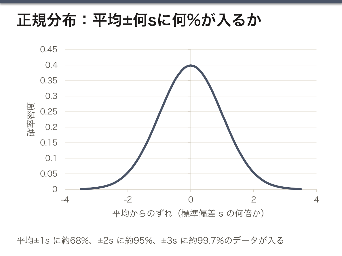
ばらつきの大きさは分散と、その平方根の標準偏差で表す。母集団全体なら σ2 = Σ(x − x̄)2/n、標本から推定するなら s2 = Σ(x − x̄)2/(n − 1)。正規分布では平均 ±1s に約68%、±2s に約95%、±3s に約99.7%のデータが入る。
なぜ標本では n − 1 で割るのか。標本の平均 x̄ は、その標本自身のデータに最もよく合うように決まった値である。だから各データから x̄ までの距離は、本当の母平均までの距離より系統的に少し短くなる。n で割るとばらつきを小さく見積もりすぎるので、n − 1 で割って補正する。実験の測定は「起こりうる全測定」の一部を取り出した標本なので、物理の測定データは標本の式(n − 1)で処理する。
なぜ測定値は正規分布になりやすいのか。小さな独立の誤差がたくさん足し合わさると、個々の誤差の形にかかわらず和は正規分布に近づく(中心極限定理)。釘の間を玉が左右にはねながら落ちるゴルトン・ボードがその実演である。
多くの検査の基準範囲は「健常者の中央95%」、つまりほぼ平均 ±2SD で決められている。裏を返すと、健康な人でも20人に1人は基準範囲の外に出る。検査項目を20個並べれば、どれか1つが外れるのはむしろ普通——「基準外=異常」ではない理由がここにある。
English version
Core
As the class width gets narrower, the histogram of many measurements approaches a symmetric bell shape, the normal (Gaussian) distribution.
f(x) = (1/σ√(2π))·exp[−(x − x̄)2/2σ2]
Spread is described by the variance and its square root, the standard deviation. For a whole population, σ2 = Σ(x − x̄)2/n; estimated from a sample, s2 = Σ(x − x̄)2/(n − 1). In a normal distribution, about 68% of the data lie within the mean ±1s, about 95% within ±2s, and about 99.7% within ±3s.
Going further
Why divide by n − 1 for a sample? The sample mean x̄ is the value that fits that sample’s own data best. So the distances from each data point to x̄ are systematically a little shorter than the distances to the true population mean. Dividing by n underestimates the spread, and dividing by n − 1 corrects it. An experiment takes only a part of “all possible measurements”, so physics data are processed with the sample formula (n − 1).
Why are measurements so often normally distributed? When many small independent errors add up, the sum approaches a normal distribution whatever the shape of each error (the central limit theorem). The Galton board, where balls bounce left and right between pins as they fall, shows this.
In the clinic
For many tests, the reference interval is “the central 95% of healthy people”, roughly the mean ±2SD. Turned around, one healthy person in twenty falls outside the reference interval. With twenty tests on one report, it is normal for one of them to be outside — this is why “outside the reference interval” does not mean “abnormal”.
平均値の信頼区間 — 標準誤差と Student の t
標準偏差 s は個々の測定値のばらつきである。これに対して平均値そのもののばらつきは標準誤差 s/√n で表す。
平均値の不確かさ(絶対誤差)Δ は、標準誤差にStudent の係数 t を掛けて求める。
Δ = tβ·s/√n
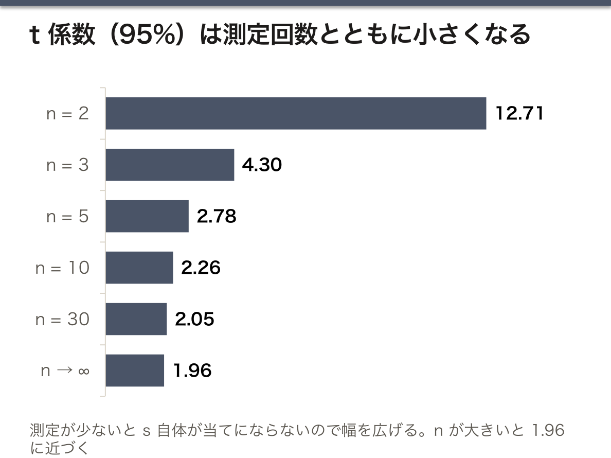
t は測定回数 n と信頼水準 β(ふつう95%)で決まる。95%なら n = 5 で 2.78、n = 10 で 2.26、n = 30 で 2.05。結果は x̄ ± Δ と書き、この幅を信頼区間という。
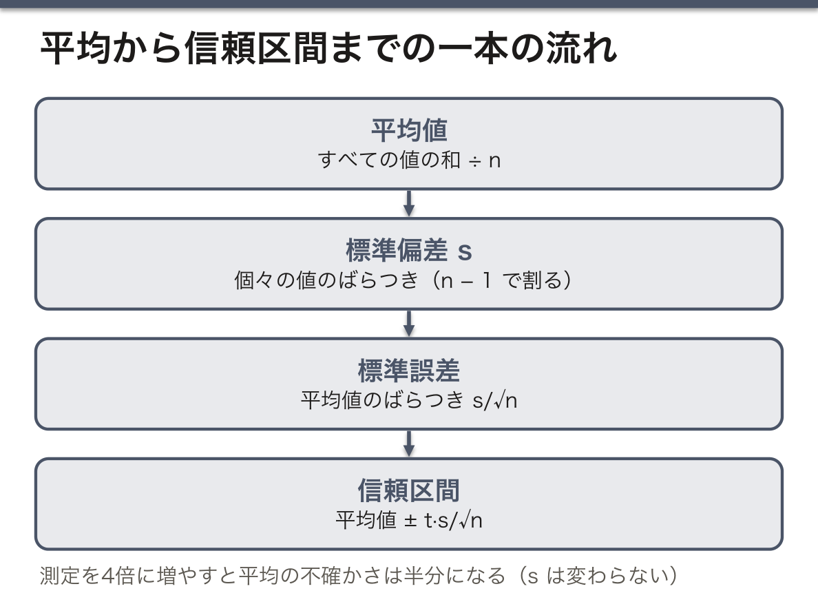
√n の意味が要点である。測定を4倍に増やすと平均の不確かさは半分になる。個々の値のばらつき s は回数を増やしても変わらない(測定法の性質だから)が、平均値はどんどん絞り込まれる。
t が n とともに小さくなる理由は、少ない測定では s 自体が当てにならないからである。5回の測定から出した s はたまたま小さく出ているかもしれない。その分を見込んで幅を広げるのが t で、n が大きくなると正規分布の値 1.96 に近づく。
例:赤血球30個の直径が平均 7.5 μm、s = 0.5 μm なら、Δ = 2.05 × 0.5/√30 ≈ 0.19 μm で、(7.5 ± 0.2) μm。
論文の図で誤差棒が SD なのか SEM なのかは必ず確かめる。SEM は SD の 1/√n なので、症例数が多いと非常に短くなり、群の差が実際より目立って見える。個々の患者のばらつきを知りたいなら SD、平均の推定の確かさなら SEM か信頼区間である。
English version
Core
The standard deviation s is the spread of individual measurements. The spread of the mean itself is the standard error, s/√n.
The uncertainty (absolute error) Δ of the mean is the standard error multiplied by Student’s coefficient t:
Δ = tβ·s/√n
t depends on the number of measurements n and the confidence level β (usually 95%). At 95%, it is 2.78 for n = 5, 2.26 for n = 10 and 2.05 for n = 30. The result is written x̄ ± Δ, and this range is the confidence interval.
Going further
The point is the √n. Four times as many measurements halve the uncertainty of the mean. The spread of single values s does not change with more measurements (it is a property of the method), but the mean is pinned down more and more.
t gets smaller as n grows because with few measurements, s itself is unreliable. An s from five measurements may be small just by chance. t widens the interval to allow for this, and as n grows it approaches the normal-distribution value of 1.96.
Example: if 30 red cells have a mean diameter of 7.5 μm with s = 0.5 μm, then Δ = 2.05 × 0.5/√30 ≈ 0.19 μm, giving (7.5 ± 0.2) μm.
In the clinic
In a figure in a paper, always check whether the error bars are SD or SEM. The SEM is 1/√n of the SD, so with many patients it becomes very short and differences between groups look larger than they are. Use the SD to see how individual patients vary; use the SEM or a confidence interval to see how well the mean is estimated.
結果の評価 — 絶対誤差・相対誤差・相対差
結果を評価する量は3つある。
| 量 | 式 | 何を見るか |
|---|---|---|
| 絶対誤差 Δ | t·s/√n(単位つき) | 平均値のばらつきの幅 |
| 相対誤差 r | Δ/x̄ × 100% | 精度を単位なしで比べる |
| 相対差 D | |x̄ − 基準値|/基準値 × 100% | 正確さ(文献値とのずれ) |
実験が理論(文献値)と合っていると言えるのは、基準値が x̄ ± Δ の区間に入るときである。
なぜ相対誤差が要るのか。±0.2 μm と ±0.2 m は同じ「0.2」でも重みがまったく違う。平均で割って割合にすれば、単位も大きさも違う測定どうしの精度を比べられる。
判定の手順は2段で考える。まず相対誤差でばらつきが小さいかを見る。次に基準値が信頼区間に入るかを見る。区間が狭いのに基準値が外れていれば、偶然では説明できない=系統誤差を疑う。逆に区間が広すぎて何でも入ってしまうなら、「合っている」と言っても意味が薄い。たとえば振り子で求めた重力加速度が (9.6 ± 0.1) m/s2 なら、9.81 は区間の外なので、振り子の長さの測り方など系統的な原因を探すことになる。
English version
Core
Three quantities are used to judge a result.
| Quantity | Formula | What it shows |
|---|---|---|
| Absolute error Δ | t·s/√n (with unit) | The width of the spread of the mean |
| Relative error r | Δ/x̄ × 100% | Compares precision without units |
| Relative difference D | |x̄ − reference|/reference × 100% | Accuracy (offset from the literature value) |
The experiment agrees with theory (the literature value) when the reference value lies inside the interval x̄ ± Δ.
Going further
Why do we need the relative error? ±0.2 μm and ±0.2 m are both “0.2” but have very different weight. Dividing by the mean turns it into a fraction, so you can compare the precision of measurements with different units and sizes.
Judge in two steps. First, use the relative error to see whether the spread is small. Next, see whether the reference value is inside the confidence interval. If the interval is narrow but the reference value is outside, chance cannot explain it — suspect a systematic error. If the interval is so wide that anything fits, saying “it agrees” means little. For example, if a pendulum gives g = (9.6 ± 0.1) m/s2, 9.81 is outside the interval, so you look for a systematic cause such as how the pendulum length was measured.
まとめ
| 測定値の書き方 — 値・不確かさ・単位の3点セット | 測定の目的は、ある物理量(測定量 measurand)について情報を得ることである。 |
|---|---|
| 誤差の種類 — 正確さと精度は別物 | 誤差は性質で3つに分ける。種類中身何が落ちるか系統誤差 systematicいつも同じ向きに同じだけずれる(校正のずれた秤、目盛を斜めから読む癖)正確さ accuracy偶然誤差… |
| データの要約 — 度数分布と3つの代表値 | たくさんの測定値は、まず度数分布にまとめる。 |
| 正規分布と標準偏差 — 母集団と標本の違い | 階級幅を細かくしていくと、多くの測定のヒストグラムは左右対称の釣鐘形、正規分布(Gauss 分布)に近づく。 |
| 平均値の信頼区間 — 標準誤差と Student の t | 標準偏差 s は個々の測定値のばらつきである。 |
| 結果の評価 — 絶対誤差・相対誤差・相対差 | 結果を評価する量は3つある。量式何を見るか絶対誤差 Δt·s/√n(単位つき)平均値のばらつきの幅相対誤差 rΔ/x̄ × 100%精度を単位なしで比べる相対差 D|x̄ − 基準… |
このノートは医学生が授業の内容を自分の言葉でまとめたもので、診療の判断に使うものではありません。誤りに気づいたらお知らせください。